Open on Github

Problem setup

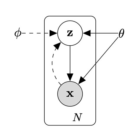
Say we want to fit a model to some data. In mathematical terms, we want to find a distribution $p$ that maximizes the probability of observed data $x \in X$. In this case, we will make the assumption that there is some latent (unobserved) variable $z$ that affects the production of $x$ behind the scenes. We can visualize this generative process in the following diagram:

This document explains methods and challenges for training latent variable models. Our end goal is to derive the variational autoencoder (VAE) [2] framework with justifications for each step along the way.

Modeling with latent variables

Our goal is to find models that fit our datapoints $x \in X$. One class of statistical models called latent variable models aims to learn about relationships between the data points (the $x$’s) and some unobserved latent variables. We often denote a latent variable with the letter $z$.

So what is a latent variable? Remember that $z$ isn’t a single number; it can be a one-dimensional vector, a two-dimensional matrix, or even something in higher dimensions. Here are some examples of what $x$ and $z$ could represent:

• $x$ is a name of a state in Canada (so $X = [“Alberta”, “Saskatchewan”, …])$. In this case, $z$ could be a single integer corresponding to a single state. This means that $z$ is a discrete variable.
• $x$ is a handwritten digit. Perhaps $z$ is a continuous vector containing compressed information about the shape of the digit. The first index of $z$ might be a measurement of how curvy the image is, the second index might indicate whether the image has a line across the top, and so on. Here, $z$ is a continuous variable.
• $x$ is a thermometer reading indicating the maximum temperature for a given day. $z$ might be a continuous variable including information the air pressure, humidity, and weather information.

Since our goal is to build a statistical model, there will rarely be a perfect choice for representation of $z$. We might even try multiple options before settling on a structure for $z$. When we make a decision about what the possible values of $z$ could be, we are choosing the prior distribution, $p(z)$.

And now that we’ve defined $p(x)$ and $p(z)$, we can also define their joint probability, $p(x,z)$. $p(x, z)$ represents the probability of a data point $x$ occurring with a specific latent $z$. Another related, subtly different distribution is the likelihood, $p(x \mid z)$, which represents the probability that some variable $x$ corresponds to a specific $z$. (Note that $p(x, z)$ = $p(x \mid z) p(z)$.)

Optimizing log p(x)

Learning with $p(x,z)$

We know each $x$ corresponds to some latent variable $z$. Although we know every $x$, we can never see $z$. This is unfortunate. The problem would be markedly easier if we could observe pairs of $(x, z)$ and jointly learn to model each $x$ and corresponding value of $z$. Because of this, we have to consider $p(x,z)$ for every possible value of $z$. In other words, we have to integrate over the distribution of possible $z$’s through a process called marginalization:

\[\log p(x) = \log \sum_{Z}p(x, z)\]

Exact marginalization

This sum is computable when there are only a few possible configurations for $z$. But as $Z$ grows, this sum quickly becomes intractable. This is because the number of possible $z$’s increases exponentially with the dimensionality of $Z$. (In programming terms, this is like a nested for loop where there is a loop corresponding to each dimension of $z$.)

This is a problem known as combinatorial explosion and makes it infeasible for us to consider iterating over every possible value of $z$. So we can’t compute $\log p(x)$ exactly. But we can approximate the sum by sampling a finite number of $z$’s. Sampling (fancy name: Monte Carlo estimation) is very helpful because it allows us to trade off computation for accuracy. Even though $Z$ is too large to enumerate, we can often sample enough values from $Z$ to approximate $\log p(x)$ with reasonable accuracy.

But where do we sample $z$ from? We want to compute $p(x,z)$ through marginalization over values of $z$, and we are okay with just approximating the solution by sampling just some values of $z$, we need to find an distribution from which we can sample values of $z$. One such distribution is the prior, $p(z)$.

The prior, $p(z)$

Remember that our goal is to maximize $\log p(x)$. We have elected to do so by approximating $p(x,z)$ by sampling $z$ values from the prior distribution $p(z)$. First, we can rewrite our marginalized quantity in terms of the prior $p(z)$ through the chain rule of probability:

\[\log \sum_{Z} p(x,z) = \log \sum_{Z} p(x \mid z) p(z)\]

Now we apply the mathematical formula known as Jensen’s inequality. Jensen’s inequality says that $f(E[x]) \geq E[f(x)]$ when $f$ is a concave function.Jensen's inequality applies in our case because $\log(x)$ is concave. Why is this true? Well, a function is concave if its second derivative is negative. If $f(x) = \log(x)$, then $f'(x) = \frac{1}{x}$, and $f"(x) = -\frac{1}{x^2}$. $-\frac{1}{x^2}$ is always negative, so $\log$ is always concave. It is very useful here because by moving the log inside the summation, we now can view our problem as an expectation with respect to the prior:

\[\begin{align*} \log (\mathbb{E}_{p(z)} p(x \mid z)) = \log \sum_{Z} p(x \mid z) p(z) &\geq \sum_{Z} p(z) \log p(x \mid z) \\ &= \mathbb{E}_{p(z)} \log p(x \mid z) \end{align*}\]

Instead of optimizing $\log p(x)$ directly (our original goal) we can instead optimize a lower bound, $\mathbb{E}_{p(z)} \log p(x \mid z)$. And since we know the prior $p(z)$ we can actually compute this quantity (or, if we’re in a hurry, we can approximate it using finite samples).

Note on lower bounds. It’s common in machine learning to maximize the evidence (in our case, the intractable $\log p(x)$) by maximizing its lower bound instead. This lower bound is often referred to as the evidence lower bound (ELBO).

Variational autoencoders (VAEs)

It’s very important to know that because of the previous step (i.e. since we invoked Jensen’s) we are no longer optimizing $\log p(x)$ directly and instead optimizing a lower bound. However, while the lower bound is convenient to optimize, in practice it may be a very loose bound (i.e. the gap between $\log p(x)$ and the lower bound $\mathbb{E}_{p(z)} \log p(x \mid z)$ could be quite large). How can we do better?

The true posterior, $p(z \mid x)$

Somewhere out there there exists a true posterior $p(z \mid x)$ that allows us to infer latent variables from our data. If we could easily obtain $p(z \mid x)$, we could use it to build a system for learning $p(x \mid z)$.

Unfortunately, if we attempt to compute $p(z \mid x)$, we run into the same problem as before: exactly computing $p(z \mid x)$ requires enumeration over the space of all possible $x$’s.This limitation can be shown via a combination of the chain rule and marginalization: $$p(z \mid x) = \dfrac{p(x, z)}{p(x)} = \dfrac{p(x,z)}{\sum_z p(x, z)}$$ Thus, the true posterior $p(z \mid x)$ relies on an intractable marginalization and we cannot compute it exactly.

Although we can’t compute $p(z \mid x)$, we can learn an approximate of it, which we call $q(z \mid x)$. $q(z \mid x)$ is a function that does inference: it produces $z$’s from $x$’s. In this context, $q(z \mid x)$ might be called the approximate posterior, variational posterior, or inference network.

The variational posterior, $q(z \mid x)$

Although we never know the true posterior $p(z \mid x)$, in practice, even its approximation $q(z \mid x)$ proves to be extremely useful. This is how (and why) variational autoencoders work: they provide a better approximation to $\log p(x)$ by learning $q(z \mid x)$.

We can think of $q(z \mid x)$ as a crutch for learning, since our end goal is still to optimize $\log p(x)$. This is where the machine learning part comes in: for some input $x$, we can sample $z \sim q(z \mid x)$, then score $\hat{x} \sim p(x \mid z)$. We can improve our model by adjusting the parameters of $q(z \mid x)$ and $p(x \mid z)$ to incrementally improve the score of $x$ given by $p(x \mid z)$.

In the world of machine learning, this type of model (learning $\log p(x)$ by jointly learning $p(x \mid z)$ and $q(z \mid x)$) is called an autoencoder. The approximate posterior $q(z \mid x)$ is called the encoder, and the likelihood $p(x \mid z)$ is called the decoder.

Finding a tighter bound

Now we need to calculate the new lower bound, the one we get when we include $q(z \mid x)$. To introduce $q(z \mid x)$ into the mix, we’ll use an old trick: multiplying by 1! Starting with $\log p(x)$, we’ll marginalize over $z$ like before, but then we’ll multiply everything by $\dfrac{q(z \mid x)}{q(z \mid x)}$:

\[\log p(x) = \log \sum_{Z} p(x \mid z) p(z) = \log \sum_{Z} \frac{q(z \mid x)}{q(z \mid x)} p(x \mid z) p(z)\]

Like in the previous section, we can use Jensen’s inequality to move the $\log$ inside the summation. And by the properties of logarithms, we can decompose the logarithm of a product into two terms:

\[\begin{aligned} \log \sum_{Z} \frac{q(z \mid x)}{q(z \mid x)} p(x \mid z) p(z) &\geq \sum_{Z} q(z \mid x) \log p(x \mid z) \frac{p(z)}{q(z \mid x)} \\ &= \sum_{Z} q(z \mid x) \log p(x \mid z) + \sum_{Z} q(z \mid x) \log \frac{p(z)}{q(z \mid x)} \end{aligned}\]

Intuition for variational autoencoders

Just like before, since we invoked Jensen’s inequality, these two terms provide a lower bound for our original quantity $\log p(x)$. We can examine each part individually:

The first term $\sum_{Z} q(z \mid x) \log p(x \mid z)$ can be rewritten as an expectation over $q$: $\mathbb{E}_{q(z \mid x)}[\log p(x \mid z)]$. This term is often called the reconstruction loss, and represents the probability the model assigns to $x$ over the distribution of $z$ that $q$ produces from $x$. If $q$ and $p$ fit the data well, then for some $z \sim q(z \mid x)$, $p(x \mid z)$ will be high. If the model is randomly initialized, $z$ will be a random code and $p(x \mid z)$ will be very low.

The second term $\sum_{Z} q(z \mid x) \log \dfrac{p(z)}{q(z \mid x)}$ can be expressed as the Kullback–Leibler divergence (often shortened to “KL divergence” or “KL”) between the posterior $q(z \mid x)$ and the prior $p(z)$. This can be written as $\mathbb{K}\mathbb{L}[q(z \mid x) \mid \mid p(z)]$ and intuitively thought of as a distance metric between the two distributions.KL doesn't technically count as a distance metric since it's not symmetric, i.e. $\mathbb{K}\mathbb{L}[(p(x) \mid \mid p(z)]$ is not always equal to $\mathbb{K}\mathbb{L}[p(z) \mid \mid p(x)]$. The KL divergence between a distribution and itself is zero.

As the approximate posterior $q(z \mid x)$ approaches the true posterior $p(z \mid x)$, the KL divergence term approaches zero. In this case, the ELBO bound becomes tight, and we are directly optimizing $\log p(x \mid z)$.

To summarize, we want to maximize $\log p(x)$, and the variational autoencoder framework provides us with a tractable lower bound to optimize. The lower bound consists of two pieces. The first term gives the probability of reproducing the data $x$ from $z$ sampled from the posterior distribution $q(z \mid x)$. The second term tells us how much the posterior distribution $q(z \mid x)$ differs from our known prior distribution $p(z)$. We want to jointly maximize the first term and minimize the second term. We can summarize this in one equation:

\[\begin{aligned} \log p(x) &\geq\overbrace{\mathbb{E}_{q(z \mid x)}[\log p(x \mid z)]}^{\text{Reconstruction loss}} - \overbrace{\mathbb{K}\mathbb{L}[q(z \mid x) \mid \mid p(z)]}^{\text{KL Divergence}} \end{aligned}\]

Gradient estimation: continuous variables

Estimating the gradient of the ELBO

We want to maximize $\log p(x)$ by maximizing its ELBO (lower bound). But our ELBO is still in the form of an expectation. We need to figure out how to rewrite these expectations into a form that we can compute, and optimize, in practice.

Although we can’t find the exact value of these expectations, we can approximate them using finite samples. For example, this is how we might use finite samples to approximate the reconstruction loss:

\[\mathbb{E}_{q(z \mid x)}[\log p(x \mid z)]\ \approx \frac{1}{N} \sum_{n=1}^{N} \log p(x \mid z^{(n)})\ \text{where}\ z^{(n)} \sim q(z \mid x)\]

This “approximation” is really just an average over $N$ samples from the distribution.

We could use finite samples to approximate the ELBO for our $q(z \mid x)$, $p(z)$, and $p(z \mid x)$. In our case, though, we don’t want to evaluate the ELBO directly. We want to find the gradient of the ELBO so that we can maximize it via stochastic gradient descent. And we run into trouble using this method of finite samples to approximate the gradient of an expectation.

Gradient estimators

Since we cannot use Monte Carlo methods to approximate the gradient of an expectation, we need to find another way to optimize the ELBO. There are various solutions proposed to compute the gradient of an expectation: these methods are known as gradient estimators. We could use any of them to solve our problem, and different choice of gradient estimators result in different tradeoffs.

There are two broad classes of gradient estimators [4]. The score function estimator, most popularly known as REINFORCE in reinforcement learning literature, could be used to solve our problem, but is notorious for producing estimates with very high variance. Instead we’re going to choose the other option, the pathwise gradient estimator, which promises lower variance. (The pathwise gradient estimator is basically better but isn’t always an option. In some cases, we have no choice but to use score function estimators like REINFORCE! This is why there is a whole field of literature around variance reduction techniques for gradient estimators. The main reason we would want to use a score function estimator is when $z$ is a discrete random variable and we aren't able to use the Gumbel-Softmax reparameterization trick like we do in this document.

Pathwise gradient estimation

The pathwise gradient estimator estimator works by re-writing the gradient of the expectation with respect to $q(z \mid x)$, which we can’t compute, as the gradient of the expectation with respect to some distribution which is independent from the rest of our model, which we can compute. This technique is known in machine learning as the reparameterization trick.

To understand why reparameterization is necessary, let’s return to the reconstruction loss:

\[E_{q(z \mid x)}[\log p(x \mid z)]\]

To train our VAE, we want to optimize (maximize) this quantity via gradient descent. We’ll first have to compute this quantity, which we now know how to do with Monte Carlo estimation:

\[\frac{1}{N} \sum_{n=1}^{N} \log p\left(x \mid z^{(n)}\right) \ \text{where}\ z^{(n)} \sim q(z \mid x)\]

Then, to perform gradient descent, we’ll have to calculate the gradient of the estimated reconstruction loss with respect to $\phi$, the parameters of our variational model. But what happens when we try differentiate this estimator with respect to $\phi$?

\[\frac{\partial}{\partial \phi} \left[\frac{1}{N} \sum_{n=1}^{N} \log p\left(x \mid z^{(n)}\right) \right]\ \text{where}\ z^{(n)} \sim q(z \mid x)\]

Unfortunately, since $z^{(n)}$ is stochastic, this quantity is non-differentiable [2]. Random sampling is considered a non-differentiable operation in mathematics. But this is where the reparameterization comes in: if we can re-write our expectation in terms of some other variable, one that isn’t part of the variational parameters, then we can differentiate, and thus we can optimize the ELBO. In the next section we’ll consider a concrete example of reparameterization, one where $z$ is Gaussian.

Gaussian reparameterization example

Let’s consider an example to make the reparameterization trick clearer. Remember we can choose any distribution we want for $z$. To illustrate reparameterization, let’s choose $z$ to be distributed as a Gaussian, i.e. $p(z \mid x) = \mathcal{N}(\mu, \sigma)$. Sampling is a non-differentiable operation, even though we want to learn $\mu$ and $\sigma$, the parameters of the distribution that defines $z$.

The reparameterization trick works like this: we can sample from a fixed distribution and then apply $\mu$ and $\sigma$ to re-create $\mathcal{N}(\mu, \sigma)$. In this Gaussian case, a very nice property holds: instead of sampling $z \sim \mathcal{N}(\mu, \sigma)$, we can say $z = \mu + \sigma \cdot \epsilon$ where $\epsilon$ is sampled from the unit Gaussian (in math, $\epsilon \sim \mathcal{N}(0,1)$).

Now the sampling operation has been moved out of the main path of the computational graph, and is done to produce $\epsilon$, which is an input to the network rather than part of the main computational path. And backpropagation works again! (This trick is what you’d actually use to train a VAE with a Gaussian latent variable.)

Gradient estimation: discrete variables

Now we know how to train a VAE with a Gaussian latent variable using the reparameterization trick. But our prior will not always tell us that the latent variable takes on a Gaussian distribution. The latent variable may indicate a class of object (perhaps a “gibbon” or “German Shepherd” image) or the index of a note on a piano (was it a C$_4$ or E$_4$?). In both of these cases, $z$ and its potential values discrete, and are parameterized by a categorical distribution.

The reparameterization worked in the Gaussian case because we had a function for sampling from the Gaussian distribution, and a way to re-write $z$ to depend on the sampled value. So we need a way to sample from the categorical distribution that allows us to re-write things so that the sampling occurs independent of any variables we might want to learn.

The Gumbel-max trick

The Gumbel-max trick provides us with an easy way to sample from a categorical distribution given the log-probabilities for each category. It’s simple: just add some Gumbel noise and take the maximum value. We can draw samples $z$ from the categorical distribution defined by class log-probabilities $\pi_i$ by adding some Gumbel noise. (In this equation, the $\texttt{one\textunderscore hot}$ function replaces the original vector with a vector of zeros with a 1 where the max is.)

\[z = \texttt{one\_hot}(\arg\max_{i}(g_i + \log \pi_i))\ \text{where}\ g_i \sim \text{Gumbel}(0, 1)\]

Applying the Gumbel-max trick is equivalent to sampling from a categorical distribution. We can express this in mathematical notation: after sampling $z$ from class probabilities $\pi_i$ using Gumbel-max, $P[z = i] = \pi_i$ (equivalently, $z \sim \text{Categorical}(\pi))$.

The Gumbel-max trick allows us to sample from a categorical distribution, but unfortunately it’s not differentiable because of the “hard” $\arg\max$ operation. Luckily, there’s a way around this.

Gumbel-Softmax

It’s a common trick in machine learning to replace a “hard” $\arg\max$ with a softmax operation in order to make a computation differentiable. The softmax function creates a probability distribution from a vector by exponentiating each value and then averaging them. This gives us an output that looks very similar to a max: in most cases, the highest value will be close to $1$ after a softmax and the other values will be close to $0$.

The typical equation for softmax looks like this:

\[\text{softmax}(x)_i = \frac{\exp{x_i}}{\sum_j{\exp{x_j}}}\]

To approximate argmax with softmax, we introduce a temperature variable $\tau$. As the temperature approaches 0, the behavior of softmax approaches that of argmax. If we replace the $\arg\max$ from our original equation with $\text{softmax}$ we get the following equation:

\[z_i = \frac{\exp{((\log \pi_i + g_i)} / \tau)}{\sum_j \exp{((\log \pi_j + g_i) / \tau})}\]

This re-writes our sampling operation in terms of $\pi_i$ (our logits, outputted by $\Phi$) and $g_i$ (sampled from the Gumbel distribution). So it’s effectively a reparameterization trick for the categorical distribution, and allows us to learn a categorical parameterization for $z$!

Both [1] and [3] proposed this solution for learning categorical latent variables.

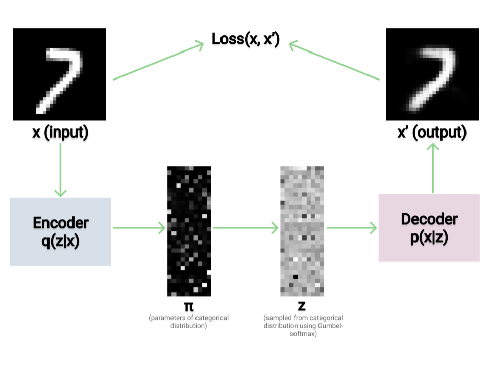
Training a little VAE

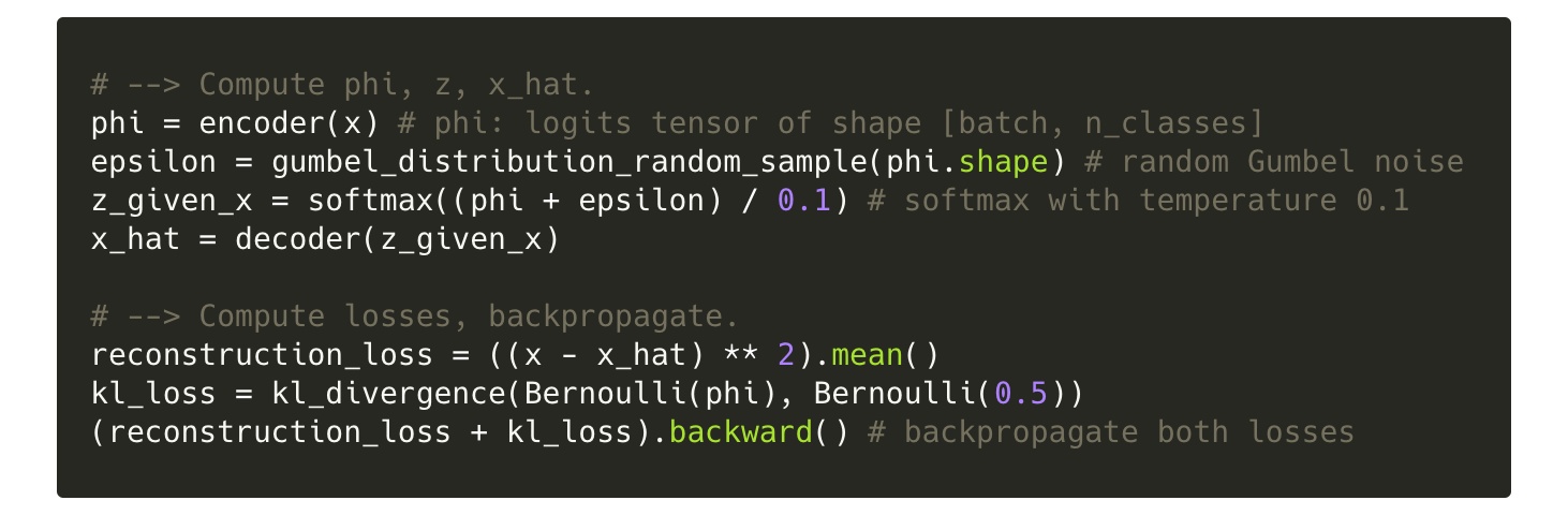
In this section we discuss how one might go about actually training a variational autoencoder where $p(x \mid z)$ and $q(z \mid x)$ are parameterized by neural networks $\theta$ and $\Phi$. The basic idea is to iterate over each $x \in X$ and compute a loss (the reconstruction loss minus the KL divergence). For each $x$, we compute this loss for a single value of $z$ sampled from $q(z \mid x)$.

We can implement this VAE in modern machine learning software libraries like TensorFlow or PyTorch. The software will automatically differentiate $\theta$ and $\Phi$ with respect to the loss and allow us to make small updates to those parameters in the directions that minimize the loss.

The process for a single step of training a categorical VAE looks like this:

1. compute $\Phi$, the parameters of $q(z \mid x)$, from $x$
2. sample $z \mid x$ from $q_{\Phi}(z \mid x)$ using the Gumbel-softmax reparameterization trick
3. compute $\hat{x}$ from $\theta$
4. compute loss $\mathcal{L}(x, \hat{x}, \Phi)$
5. use auto-differentiation to update $\Phi$ and $\theta$ based on $\mathcal{L}$

Conclusion

Hopefully, this tutorial improved your intuitions for latent variable models and variational autoencoders, especially in the case where the latent variables $z$ are discrete. The following section summaries some of the most important math that’s useful for this sort of thing. It may be a helpful reference when learning more about latent variable models, variational autoencoders, etc.

Useful mathematical definitions

(1) Bayes’ theorem: $p(x \mid z) = \dfrac{p(z \mid x)p(x)}{p(z)}$

(2) Bayesian terminology:

• likelihood $p(x \mid z)$
• evidence $p(x)$
• posterior $p(z \mid x)$
• prior $p(z)$

(3) Jensen’s inequality: $\phi(E[X]) \leq E[\phi(X)]$ where $\phi$ is a convex function.

(4) Law of the unconscious statistician. A good rule of thumb: any time you see a sum and a probability distribution inside the sum, you should interpret it as an expectation of whatever else is in that sum with respect to that probability distribution. For discrete variables:

\[E[g(X)] = \sum_x g(x) p(x)\]

where $p(x)$ is the probability mass function of discrete random variable $x$. And for continuous variables:

\[E[g(x)] = \int_{-\infty}^{\infty} g(x) p(x) dx\]

where p(x) is the probability density function of continuous random variable $x$. (This is also the definition of an expectation.)

(5) Marginalization. Say we have a joint distribution $p(x,y)$ for two random variables $X$ and $Y$, but we want to obtain a marginal distribution for $X$, the probability distribution $p(x)$ where $Y$ is not taken into consideration. We can find this by summing (or, in the case of a continuous variable, integrating) over all values of $Y$:

\[p_X(x) = \sum_j p(x, y_j)\]

(6) KL divergence is a measure of how one probability distribution differs from another:

\[\mathbb{K}\mathbb{L}[p(x), q(x)] = \sum_{x \in X} p(x) \log \dfrac{p(x)}{q(x)}\]

(Note that $\mathbb{K}\mathbb{L}[p(x), q(x)] \neq \mathbb{K}\mathbb{L}[q(x), p(x)]$.)

(7) The Gumbel distribution is a distribution used to model the maximum (or minimum) value of a distribution. The Gumbel-max trick is a way to sample from categorical distributions.

(8) The softmax function performs exponentiation and an average over a vector, which often looks like a smoothed version of the maximum value. Softmax can be calculated with a temperature constant – a higher temperature smooths the output of the softmax, while a temperature close to 0 makes the softmax spikier, bringing it closer to a true argmax.

Acknowledgements

Thanks to Justin Chiu, Keyon Vafa, and Yuntian Deng for comments and suggestions on how to improve this tutorial.

References

1. Eric Jang, Shixiang Gu, and Ben Poole. Categorical reparameterization with gumbel-softmax, 2017.

2. Diederik P Kingma and Max Welling. Auto-encoding variational bayes, 2014.

3. Chris J. Maddison, Andriy Mnih, and Yee Whye Teh. The concrete distribution: A continuous relaxation of discrete random variables. CoRR, abs/1611.00712, 2016.

4. John Schulman, Nicolas Heess, Theophane Weber, and Pieter Abbeel. Gradient estimation using stochastic computation graphs. CoRR, abs/1506.05254, 2015