![]()
Introduction
This document describes two machine learning methods, Noise Contrastive Estimation (NCE) [5] and its follow-up InfoNCE [15]. We discuss two variants of NCE as well as InfoNCE and a related technique called partition function estimation. NCE-based methods are used for estimating the parameters of a statistical distribution by differentiating between “real data” and “noise”.
We will try to keep our terminology consistent. The original NCE method is sometimes referred to as Local NCE [3,13] or Binary NCE . We’ll call it Local NCE. The follow-up InfoNCE is very similar to an NCE variant called both Global NCE [13] and Ranking NCE [8], which we’ll call Global NCE.
Applications. Local NCE and Global NCE are both computationally inexpensive methods for learning a conditional likelihood $p_\theta(x \mid c)$. NCE is useful in general when the number of possible $x$’s is very large, like in language modeling [6,8], where $|X|$ is the number of words in a vocabulary. InfoNCE is a method for maximizing the mutual information between two variables, which forms the foundation of joint text-to-image learning methods like CLIP [11], where $x$ is an image and $c$ the text of its caption, as well as general contrastive learning-based techniques like SimCLR [1], where $x$ and $c$ are two different ‘views’ of the same image.
Overview. We begin by discussing how NCE works to approximate $p(x \mid c)$. We then consider how we could approximate $p(x \mid c)$ via importance sampling, a method sometimes known as partition function estimation. Then we connect partition function estimation to Global NCE and InfoNCE. We end with discussion of the differences between the methods and suggestions for which to use in practice.
What are x and c?
Local NCE and Global NCE focus on learning $p(x \mid c)$, the likelihood of some $x$ given some ‘context’ $c$. InfoNCE maximizes $\frac{p(x \mid c)}{p(x)}$, a proxy for mutual information between $x$ and $c$. But what are $x$ and $c$ anyway? Here are examples of x’s and c’s from the literature:
- In NLP: Local NCE and Global NCE are both used for language modeling, where $x$ is a word and $c$ is the word’s context (the other words in a window around $x$). Here, we want to learn $p(x \mid c)$, the probability of the next word given context. [6]
- In speech recognition: Local NCE is used for learning $p(x \mid c)$ where $x$ is a word predicted from audio $c$ in which the word was spoken. [18]
- Also in speech recognition: InfoNCE is used to maximize the mutual information between representations of the same word in different contexts. Here, $x$ is a word and $c$ is the audio context. [19]
- In reinforcement learning: InfoNCE is used as a regularizer, where $x$ and $c$ are representations of the same game state at different times. Here, we want to maximize the mutual information between $x$ and $c$, which is proportional to $\frac{p(x \mid c)}{p(x)}$. [16]
- In computer vision: InfoNCE is used for contrastive learning, where $x$ and $c$ are different views (different crops with random augmentations like color filters and image-stretching applied) of the same image, and we again want to maximize the mutual information between $x$ and $c$. [1]
- In generative adversarial networks (GANs): Local NCE is similar to the ‘discriminator’ of a GAN, except that with a GAN, the ‘generator’ $q(x)$ is learned, and with Local NCE the generator $q(x)$ is fixed throughout training. [17]
Local NCE
How can we estimate $p_{\theta}(x \mid c)$ where $c$ is some context and $x$ is one of a large number of classes? We can rewrite the objective like this:
\[p_{\theta}(x \mid c) = \dfrac{f_\theta (x, c)}{\sum_{x'} f_\theta (x', c)} = \dfrac{f_\theta (x, c)}{Z_\theta (c)}\]where $f_\theta(x, c)$ assigns a score to $x$ in context and $Z_\theta (c)$ is the normalizing constant or partition function. $Z$ is difficult to compute in this case of many possible classes, because we have to sum over every possible $x’$.
Local NCE reduces the problem of learning $p_\theta(x \mid c)$ to learning a binary classifier $p(d \mid x, c)$, where $d$ tells us whether data point $c$ is “real”, i.e. sampled from $p(x \mid c)$, rather than “noise”, sampled from some noise distribution $q(x)$. Technically, $d$ is an indicator variable where $[d=0]$ implies that $x \sim q(x)$.
In Local NCE, we sample $k$ real samples (or negative samples) from $q(x)$ and assign them the label $D=0$. We sample one true data point (or positive sample) from $p(x \mid c)$. We can write the conditional probability of $d$ having observed $x$ and $c$:
\[\begin{align*} p(D = 0 \mid x, c) &= \dfrac{k \cdot q(x)}{p(x \mid c) + k \cdot q(x)} \\ p(D = 1 \mid x, c) &= \dfrac{p(x \mid c)}{p(x \mid c) + k \cdot q(x)} \end{align*}\]Now we want to write these probabilities in terms of the scoring function $f_\theta$. Local NCE typically makes a key assumption that we can assume $Z_\theta(c) \approx 1$; this assumption is called self-normalization and tends to work well in practice, since neural networks are expressive enough to learn self-normalized scoring functions.
Self-normalization implies that $p(x \mid c) = f_\theta (x, c)$. With this assumption, we can rewrite the conditional likelihood in terms of $f_\theta$:
\[\begin{align*} p(D = 0 \mid x, c) &= \dfrac{k \cdot q(x)}{f_\theta(x,c) + k \cdot q(x)} \\ p(D = 1 \mid x, c) &= \dfrac{f_\theta(x,c)}{f_\theta(x,c) + k \cdot q(x)} \end{align*}\]This is a typical binary classification problem: learn a $\theta$ that maximizes the conditional log-likelihood of $p(D \mid x, c)$. So we can write the loss as the binary classification error:
\[\begin{equation} \mathcal{L}_{\text{LocalNCE}} = \sum_{(x, c) \in D} \left[ \\ \log p(D = 1 \mid x, c) \\ + k \mathbb{E}_{x' \sim q} \log p(D = 0 \mid x', c) \right] \end{equation}\]This loss $\mathcal{L}_{\text{LocalNCE}}$ isn’t actually useful yet because it still requires computing an expectation over $q(x)$, which would still loop over all possible classes for $x$! So, finally, we approximate the inner expectation Monte-Carlo sampling, using $k$ samples from $q(x)$:
\[\begin{equation*} \mathcal{L}_{\text{LocalNCE,MC}} = \sum_{(x, c) \in D} \left( \log p(D = 1 \mid x, c) + \sum_{i=1, x' \sim q}^{k} \log p(D = 0 \mid x', c) \right) \end{equation*}\]The original NCE paper [5] shows how, as $k \rightarrow \infty$, the gradient of $\mathcal{L}$ is only zero once $f_\theta(x, c) = p(x \mid c)$. See the appendix for more detail.
So the main idea is that we can optimize $p(D \mid x, c)$ instead of $p(x \mid c)$, and the self-normalized scoring function we learn $f_\theta (x \mid c)$ will approximate $p_\theta(x \mid c)$.
Application: Negative sampling
NCE gives us a way to learn $f(x, c) \approx p(x \mid c)$ without computing the partition function, which can be expensive or even intractable. But it still requires some engineering; in particular, we have to choose $k$, the number of noise examples, and $q(x)$, the noise distribution.
Let’s choose some reasonable defaults for these parameters in the case of language modeling. We might choose $k=|V|$, so the probability of choosing a real point (as opposed to noise) is roughly $\frac{1}{|V|}$. And (without any prior knowledge of language) it seems reasonable to set $q(x)$ to a uniform distribution over the vocabulary, i.e. $q(x) = \frac{1}{|V|}$.
Given these choices for $k$ and $q$, we can simplify the NCE objective:
\[\begin{equation*} p(D = 0 \mid x, c) = \dfrac{ |V \mid \cdot \frac{1}{|V|} }{f_\theta(x,c) + |V \mid \cdot \frac{1}{|V|}} = \dfrac{1}{f_\theta(x,c) + 1} \end{equation*}\] \[\begin{equation*} p(D = 1 \mid x, c) = \dfrac{f_\theta(x,c) }{f_\theta(x,c) + |V \mid \cdot \frac{1}{|V|}} = \dfrac{f_\theta(x,c) }{f_\theta(x,c) + 1} \end{equation*}\]This variation of NCE with $k = |V|$ and $q(x) = \frac{1}{|V|}$ is used in negative sampling [9,4], the method underlying the popular word2vec algorithm.
Approximating Z
Another way to learn $p(x \mid c)$ is to directly approximate it via sampling. When deriving NCE, we noted that:
\[\begin{equation*} p_\theta(x \mid c) = \dfrac{f_\theta(x, c)}{Z_\theta(c)} \end{equation*}\]And with NCE, we avoided computing the partition function $Z$ by forcing the scoring function $f$ to “include” the partition function, via self-normalization. Suppose that instead of avoiding computing the partition function (by forcing the model to self-normalize) we decided to approximate $Z$ by sampling $x \sim q(x)$ $k$ times:
\[\begin{align*} Z_\theta(c) = \sum_j f_\theta(x_j, c) &= \sum_j f_\theta(x_j, c) \dfrac{q(x_j)}{q(x_j)} \\ &= \mathbb{E}_{x_j \in X} \left[ \dfrac{f_\theta(x_j, c)}{q(x)} \right] \\ &\approx \sum_{j=1, x_j \sim q(x)}^{k}\dfrac{f_\theta(x_j, c)}{q(x_j)} \end{align*}\]This type of approximation via sampling from $q(x)$ is called importance sampling. We can plug the approximation of $Z_\theta$ in to approximate the conditional likelihood:
\[\begin{equation} p(x \mid c) \approx \dfrac{f_\theta(x, c)}{\sum_{j=1, x_j \sim q(x)} {f_\theta (x_j, c) / q(x_j)}} \end{equation}\]Note that the approximation done here is in computing $Z_\theta(x, c)$, which is why this approach is also called partition function estimation.
Global NCE
Given Equation 2, one way to learn $f$ would be via maximum likelihood estimation to directly maximize $p(x \mid c)$. However, in our case, we don’t know the true value of $p(x \mid c)$, or it’s too expensive to compute directly. So, as with Local NCE, we need to consider some surrogate objective to help us learn $p(x \mid c)$ in the setting where we can sample from $p(x \mid c)$, but can’t evaluate it directly.
Global NCE / Ranking NCE
So how can we find a surrogate objective? With Local NCE, we created a binary classification task where the classifier determines whether some $x$ came from context $p(x \mid c)$ or noise $q(x)$. The insight behind Global NCE is very similar. With Global NCE, the classifier identifies the real data point from multiple examples $x_1, …, x_k$ where one data point $x_i \sim p(x \mid c)$ is real and the remaining data points $x_{j \neq i} \sim q(x)$ are noise.
With these $x$’s, let’s create a categorical indicator variable $d$ where $[d = i]$ tells us that $x_i$ is the positive example. Then we can use $d$ to write the following objective, which is the cross-entropy of identifying the real example correctly (see the appendix for a proof):
\[\begin{align} p(d = i \mid x_i, c; k) &= \dfrac {p(x_i \mid c) \prod_{l \neq i} p(x_l)} {\sum_{n=1}^{k} p(x_n \mid c) \prod_{l \neq k} p(x_l)} \\ &= \dfrac { \frac{p(x_i \mid c)}{p(x_i)} } { \sum_{j=1}^{k} \frac{p(x_j \mid c)}{p(x_j)} } \end{align}\]Finally, we want to maximize $p(d = i \mid X, c)$ with respect to the training data, which is equivalent to maximizing $\log p(d = i \mid X, c)$. Let’s define a new scoring function $g$ where $g_{\theta}(x_i, c)$ gives us a score for how well $x_i$ fits context $c$:
\[\begin{equation*} g_\theta(x, c) \propto \dfrac{p(x \mid c)}{q(x)} \end{equation*}\]
A ratio of probabilities is sometimes referred to as a density ratio. We can rewrite $p(d = i \mid X, c)$, the probability that $x_i$ is the positive example, in terms of the newly-defined $g$:
\[\begin{align} p(d = i \mid X, c) &\approx \dfrac {g_{\theta}(x_i, c)} {\sum_{j=1}^{k} g_{\theta}(x_j, c) } \end{align}\]Note that this looks very similar to the approximation of $p(x \mid c)$ using importance sampling. The difference is that for Global NCE, the score function $g$ approximates the density ratio $\frac{p(x \mid c)}{q(x)}$, while we previously used a score function $f$ to approximate $p(x \mid c)$ directly. Both Global NCE and the importance sampling approach sample from $q(x)$ to approximate the partition function.
Given the conditional probability from Equation 4, we can define the loss for this objective:
\[\begin{align} \mathcal{L_{\text{GlobalNCE}}} = \sum_{(x_1, ..., x_k, c) \in D}\left[ \log \dfrac { g_\theta(x_i, c) } { \sum_{j} {g_\theta(x_j, c))} } \right] \end{align}\]This quantity is the cross-entropy of identifying the positive example $x_i \sim p(x \mid c)$ correctly. $\mathcal{L}_{\text{GlobalNCE}}$ is the common training objective used in Ranking NCE, Global NCE, and InfoNCE. Both NCE losses are shown to converge to $p(x \mid c)$ with the same error as maximum likelihood estimation as $k \rightarrow \infty$ [8].
Recovering $p(x \mid c)$ from $g$
The Global NCE objective is typically used to learn a useful scoring function that can be used to estimate $p(x \mid c)$ after training. If we know $q(x)$, we can define $g$ in terms of $q(x)$:
\[\begin{equation*} g_\theta(x, c) = \dfrac{h_\theta(x, c)}{q(x)} \end{equation*}\]This defines another scoring function, $h$, that directly approximates $p(x \mid c)$. Since $g_\theta(x, c) \propto \frac{p(x \mid c)}{q(x)}$, then we can see $h_\theta(x, c) \propto p(x \mid c)$. Note again that this approach requires knowing $q(x)$. So, as with Local NCE, Global NCE requires the ability to query $q(x)$ to estimate $p(x \mid c)$.
Ranking NCE methods use $q(x)$ during training in this way to approximate $p(x \mid c)$ with a scoring function. InfoNCE methods don’t use $q(x)$ and instead approximate it as part of the ratio $\frac{p(x \mid c)}{q(x)}$.
InfoNCE
Unlike the other NCE variants we’ve seen, the goal of InfoNCE is not to estimate $p(x \mid c)$ at all. Thus, InfoNCE does not require knowledge of the underlying noise distribution $q(x)$. InfoNCE shows that by learning the density ratio between $p(x \mid c)$ and $q(x)$, the Global NCE loss maximizes $I(x_i; c)$, the mutual information between data point $x_i$ and its context $c$, and minimizes $I(x_{j \neq i}; c)$.
Mutual information. The mutual information between two random variables is a measure of how dependent they are on one another. If two variables are totally independent, they have a mutual information of zero. Mutual information between two random variables $x$ and $c$ is defined as:
\[\begin{equation} \begin{aligned} I(x; c) &= \sum_{(x, c)}{ p(x, c) \log{\dfrac{p(x \mid c)}{p(x)}}} \\ &= \mathbb{K}\mathbb{L}( p(x,c) \mid \mid p(x) p(c) ) \end{aligned} \end{equation}\]Remember that if $x$ and $c$ are independent, then $p(x,c) = p(x) p(c)$. So in this case, $\mathbb{K}\mathbb{L}( p(x,c) \mid \mid p(x) p(c) )$, and thus mutual information, must be zero.
If we were to minimize the mutual information between $x$ and $c$, then, we would want that KL to go to zero – we’d be encouraging their independence. On the other hand, if we were to maximize their mutual information, we would be encouraging them to be as dependent as possible – or convey as much of the same information as one another as possible.
InfoNCE, mutual information, and contrastive learning
Recall that InfoNCE models the density ratio $g_{\theta}(x, c) = \frac{p(x \mid c)}{q(x)}$. $I(x; c) \propto \frac{p(x \mid c)}{p(x)}$, so if we make the assumption that $q(x) = p(x)$, then we can see from Equation 6 that maximizing $g_\theta(x, c)$ is equivalent to maximizing $I(x; c)$. Essentially, $g_\theta(x, c)$ will be high when $x$ comes from the context of $c$ and low when $x$ and $c$ are unrelated.
This perspective of mutual information unlocks a very powerful and general tool. Given a set of datapoints where some data are related and some aren’t, we can learn a function $g_\theta(x, c)$ that is high when $x$ and $c$ are related and low when $x$ and $c$ are unrelated. This is the essence of the field of contrastive learning, where InfoNCE underlies some of the most successful learning algorithms [1, 2, 7].
Historical note: who invented Global NCE?
[14] proposed a method called Maximum Likelihood Mutual Information to directly estimate mutual information between variables, unrelated to later NCE work. [6] was the first to adapt NCE to the multiclass classification case and touched on the connection between partition function estimation, importance sampling, and NCE. In metric learning, the idea of contrasting one positive pair against $k-1$ negative pairs was first suggested by [12]. The main contribution of the InfoNCE paper [15] is the connection between NCE and mutual information, and the use of InfoNCE to create a new unsupervised learning algorithm called Contrastive Predictive Coding.
Summary
Local NCE, Global NCE, and InfoNCE are all algorithms based on the principle of discriminating real from fake examples. InfoNCE and Global NCE are similar, but Global NCE uses $q(x)$ to estimate $p(x \mid c)$, and InfoNCE doesn’t use $q(x)$ and instead estimates $\frac{p(x \mid c)}{q(x)}$.
The training objectives are similar too:
- Local NCE: Given one data point, infer if it’s real or noise.
- Global NCE / InfoNCE: Infer which of $k$ data points is real.
Both techniques require the ability to sample from both $p(x \mid c)$ and $q(x)$. Both can be used to approximate the conditional likelihood $p(x \mid c)$, which saves computation time during training. Both are shown to approximate the log-likelihood of the data under $p$ as the number of neighbors $k \rightarrow \infty$ [8].
The methods have a few major differences:
- Assumptions. InfoNCE learns to discriminate real data from noise without knowing $q(x)$. However, the connection to mutual information only holds if $q(x) = p(x)$. Local and Global NCE work with any $q(x)$.
- Scoring function. InfoNCE and Ranking NCE model $g_\theta(x, c) \propto \frac{p(x \mid c)}{q(x)}$. If $q(x)$ is known, then the conditional likelihood can be directly modeled as $p(x \mid c) \propto q(x) \cdot f_\theta(x, c)$. Local NCE directly models $f_\theta(x, c) = p(x \mid c)$.
- Self-normalization. Global NCE maximizes $\frac{f_\theta(x,c)}{\sum_{x’} f_\theta(x’, c)}$. Local NCE directly maximizes $f_\theta(x,c)$ and minimizes $f_\theta(x’, c)$ for all $x’ \neq x$. Thus, unlike Global NCE, Local NCE is self-normalized – i.e. in Local NCE $f_\theta(x,c) \approx p_\theta(x,c)$, while in Global NCE $h_\theta(x,c) \propto p_\theta(x, c)$.
Applications
NCE was originally proposed in 2010 [5] and [10] suggested its usefulness for language modeling. Later, [6] proposed the ranking-based version of NCE, which is equivalent to InfoNCE. NCE was helpful for language modeling because directly computing $p(x \mid c)$ over every word in a language can be very computationally expensive. However, the number of words in a typical language is typically on the order of tens of thousands. As of this writing (early 2022) vocabularies don’t feel that big anymore, and it isn’t so crazy to directly compute $p(x \mid c)$, so using NCE for language modeling isn’t typically necessary.
As mentioned previously, InfoNCE can be useful for maximizing the mutual information between some datapoints in an unsupervised way. Recently, this is most common in contrastive learning for computer vision. Depending on the algorithm, the images with high mutual information might be two crops from the same image, or versions of the same image with different color transformations applied to them. In this case, the context $c$ might be a crop from an image, and $f_\theta(x,c)$ scores whether or not $x$ is a crop from the same original image as $c$.
One recent application of InfoNCE is for multimodal models that learn to produce images from text captions, and to write text captions for images. These models maximize the mutual information between images and text descriptions of those images. For example, CLIP [11] used the InfoNCE loss to learn relationships between millions of $(\text{image}, \text{caption})$ pairs scraped from the Web.
Local NCE is closely related to Generative Adversarial Networks (GANs). Local NCE can be interpreted as the ‘discriminator’ side of a GAN where the generative network ($q(x)$ in Local NCE) is fixed. [17]
Which method should I use for my problem?
First, make sure that NCE and InfoNCE are good options for your problem in the first place. If you have a distribution of related datapoints, $p(x \mid c)$, and a distribution of unrelated datapoints, $q(x)$, then these methods might be for you. Either Global NCE or Local NCE can be useful to reduce the computational complexity of learning $p(x \mid c)$, and InfoNCE can be used for learning representations for data from completely unknown distributions.
Do you have $q(x)$? If you don’t have $q(x)$, you can’t use NCE. However, you can still use InfoNCE! This is how lots of contrastive learning methods work. They learn the ratio $\frac{p(x \mid c)}{q(x)}$, which creates useful representations on its own. (But they still can’t compute the likelihood $p(x \mid c)$ without knowing $q(x)$.)
Do you have $q(x)$ and want to approximate $p(x \mid c)$? In this case, both InfoNCE or NCE will work! So which one is better? [8] suggests that if the model is complex enough to model the partition function, Global NCE is better than Local NCE, but only when the model is regularized to produce scores that are self-normalized.
Implementation
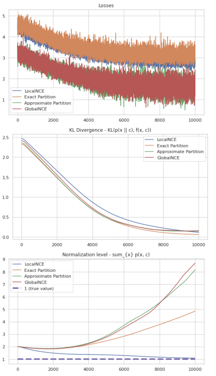
To accompany this blog post I’ve coded minimal implementations of the algorithms discussed in this post to approximate a conditional likelihood - Local NCE, Global NCE, and approximate partition function. I also added the exact partition function loss for reference. The code is in this colab notebook. We can see in the following figure how all four solutions converge to the correct distribution (shown by a very low KL), and Local NCE finds a solution that is self-normalized.
Acknowledgements
Thanks to Justin Chiu, Sasha Rush, David Noursi, Wenting Zhao, Celine Lee, and Woojeong Kim for helpful feedback and comments on this blog post.
References
- T. Chen, S. Kornblith, M. Norouzi, and G. E. Hinton. A simple framework forcontrastive learning of visual representations. ArXiv, abs/2002.05709, 2020a.
- T. Chen, S. Kornblith, K. Swersky, M. Norouzi, and G. Hinton. Big self-supervised models are strong semi-supervised learners, 2020b.
- C. Dyer. Notes on noise contrastive estimation and negative sampling. CoRR,abs/1410.8251, 2014. URL http://arxiv.org/abs/1410.8251.
- Y. Goldberg and O. Levy. word2vec explained: deriving mikolov et al.’s negative-sampling word-embedding method, 2014.
- M. U. Gutmann and A. Hyv ̈arinen. Noise-contrastive estimation: A new estimation principle for unnormalized statistical models. In AISTATS, 2010.
- R. J ́ozefowicz, O. Vinyals, M. Schuster, N. M. Shazeer, and Y. Wu. Exploring the limits of language modeling. ArXiv, abs/1602.02410, 2016.
- P. Khosla, P. Teterwak, C. Wang, A. Sarna, Y. Tian, P. Isola, A. Maschinot, C. Liu, and D. Krishnan. Supervised contrastive learning. ArXiv,abs/2004.11362, 2020.
- Z. Ma and M. Collins. Noise contrastive estimation and negative sampling for conditional models: Consistency and statistical efficiency. In EMNLP, 2018.
- T. Mikolov, K. Chen, G. Corrado, and J. Dean. Efficient estimation of word representations in vector space, 2013.
- A. Mnih and Y. W. Teh. A fast and simple algorithm for training neural probabilistic language models. In ICML, 2012.
- A. Radford, J. W. Kim, C. Hallacy, A. Ramesh, G. Goh, S. Agarwal, G. Sastry, A. Askell, P. Mishkin, J. Clark, G. Krueger, and I. Sutskever. Learning transferable visual models from natural language supervision. CoRR, abs/2103.00020, 2021. URL https://arxiv.org/abs/2103.00020.9.
- K. Sohn. Improved deep metric learning with multi-class n-pair loss objective. In NIPS, 2016.
- K. Stratos. Noise contrastive estimation, 2021.
- T. Suzuki, M. Sugiyama, J. Sese, and T. Kanamori. Approximating mutual information by maximum likelihood density ratio estimation. In FSDM, 2008.
- A. van den Oord, Y. Li, and O. Vinyals. Representation learning with contrastive predictive coding. CoRR, abs/1807.03748, 2018. URL http://arxiv.org/abs/1807.03748.
- Anand, A., Racah, E., Ozair, S., Bengio, Y., Côté, M., & Hjelm, R.D. (2019). Unsupervised State Representation Learning in Atari. ArXiv, abs/1906.08226.
- Goodfellow, I.J. (2015). On distinguishability criteria for estimating generative models. arXiv: Machine Learning.
- X. Chen, X. Liu, M. J. F. Gales and P. C. Woodland, “Recurrent neural network language model training with noise contrastive estimation for speech recognition,” 2015 IEEE International Conference on Acoustics, Speech and Signal Processing (ICASSP), 2015, pp. 5411-5415, doi: 10.1109/ICASSP.2015.7179005.
- Kawakami, K., Wang, L., Dyer, C., Blunsom, P., & Oord, A.V. (2020). Learning Robust and Multilingual Speech Representations. FINDINGS.
Extra material
Asymptotic analysis
One intuition for the Local and Global NCE losses is to think of them as sample-based approximations to the true gradient of the log-likelihood $\log p(x \mid c)$, each using $k$ examples. This means that, as $k \rightarrow \infty$, the gradients of the surrogate losses, $\frac{\partial}{\partial \theta} \mathcal{L}$ should tend towards the gradient of the log-likelihood of the data.
We can show this individually for each method:
Local NCE
\[\begin{equation*} \mathcal{L}_{\text{LocalNCE}} = \sum_{(x, c) \in D} \left[ \log p(D = 1 \mid x, c) + k \mathbb{E}_{x' \sim q} \log p(D = 0 \mid x', c) \right] \end{equation*}\]We begin by computing the gradient of the Local NCE loss (Equation 1) with respect to $\theta$:
\[\begin{equation*} \dfrac{\partial}{\partial \theta} \mathcal{L}_{\text{LocalNCE}} \\= \sum_{(x', c) \in D} \left[ \sum_{x \in V} \dfrac{k \cdot q(x)}{f_\theta(x, c) + k \cdot q(x)} (p(x \mid c) - f_\theta(x, c))\dfrac{\partial}{\partial\theta}\log f_\theta(x, c) \right] \end{equation*}\]As $k \rightarrow \infty$, the term on the left tends to 1, and we are left with:
\[\begin{equation*} \lim_{k \rightarrow \infty} \mathcal{L}_{\text{LocalNCE}} = \sum_{(x', c) \in D} \sum_{x \in V} (p(x \mid c) - f_\theta(x, c)) \dfrac{\partial}{\partial\theta}\log f_\theta(x, c) \end{equation*}\]Now we can see how the gradient (and therefore the loss) will only be zero when $f_\theta(x, c) = p(x \mid c)$.
Ranking NCE
As shown previously, Ranking NCE is analogous to sample-based approximation of the density ratio $\frac{p(x \mid c)}{q(x)}$. Thus, as $k \rightarrow \infty$ the Ranking NCE estimate $h_theta(x, c)$ converges to a value proportional to $p(x \mid c)$.
InfoNCE Proof
This is an explanation of the proof in Section 2 of the InfoNCE paper [15]:
\[\begin{align*} p(d = i \mid X, c) &= \dfrac { p(x_i \mid c) \prod_{l \neq i} p(x_l) } { \sum_{j=1}^{k} { p(x_j \mid c) \prod_{l \neq j} p(x_l) } } \\ &= \dfrac { \dfrac {p(x_i \mid c)} {p(x_i)} } {\sum_{j=1}^{k} { \dfrac {p(x_j \mid c)} {p(x_j)} } } \end{align*}\]The big fraction in the first line is a long way of writing out the cross-entropy loss: the probability that $x_i$ is the positive sample, and every other $x_l$ (where $l \neq i$) is a negative sample.
The second line is just a simplification. The product in the numerator cancels out with the product in the denominator:
\[\begin{align*} \dfrac {\prod_{l \neq i} p(x_l)} {\prod_{l \neq j} p(x_l)} = \dfrac {\frac{\prod_l p(x_l)}{p(x_i)}} {\frac{\prod_l p(x_l)}{p(x_j)}} = \dfrac {\frac{1}{p(x_i)}} {\frac{1}{p(x_j)}} \end{align*}\]To summarize this two-line proof: the first line expands out the probability distribution $p(d = i \mid X, c)$ we’re learning via optimizing $\mathcal{L}_{\text{InfoNCE}}$. The second line uses a trick to rearrange things so that the numerator is $\frac {p(x_i \mid c)}{p(x_i)}$. This equation is the quantity we wanted to optimize for, since it’s proportional to the mutual information between $x_i$ and $c$.
Maximizing mutual information in both directions
Note that, like the equation for KL divergence, $I(x,c)$ is asymmetric: $I(x;c) \neq I(c; x)$. In the case of Contrastive Predictive Coding [15], it makes sense to only maximize mutual information in one direction. The observation $x_{t+k}$ should add as little new information as possible to the context $c$. On the other hand, we don’t want to maximize $I(c,x)$ or we’d be enforcing that the context $x_t$ should only carry information that can be re-gathered at step $x_{t+k}$. In essence, the information at a single timestep should be a subset of the information gathered from multiple timesteps.
In other cases, though, we might want to maximize both $I(x, c)$ and $I(c, x)$. One case of this is in CLIP [11], where they want to learn a joint distribution such that an image and its caption share as much information as possible. In CLIP, their loss function is the sum of two terms, where each is maximizing the mutual information in one direction.